Visualize Results
Physical displacements and stresses are calculated for parts or assemblies relative to the global coordinate system for the file. You view the results of these calculations through the Results node in the browser.
Within the Results browser node are the various result nodes. You can view Stress, Strain, Displacement, Safety Factor, and Contact Pressure results.
Additional commands for evaluating the results include:
- The ability to view the mesh overlaid on the results
- Minimum and maximum views that quickly show the locations of load extremes
- A deformation adjustment that allows you to visually enhance the effects of loads so you can more readily view the impact of loads
- Volume plots, both smooth shaded and contour
- Animation of the displacement
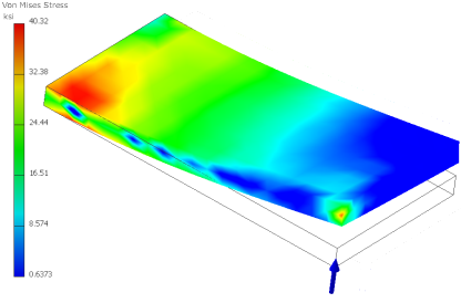
For Static Stress Analysis, you can view:
- Strain results, including the strain tensor and the Principal and Equivalent strains
- Contact pressure (tractions)
- Displacement
- Stress
- Safety Factor
Fully defined material properties must be specified for the results plots to have meaningful content. You can use the Style and Standard Editor to review the properties of any material. The Style and Standard Editor is accessible from the Assign Materials dialog box.
Design constraints can be geometry based:
- Mass and volume
- A displacement component
- A stress component
- Other applicable field data
- Safety Factor
The stress state is calculated for a part or assemblies of parts. From the elasticity theory, the three-dimensional stress state on an infinitesimal volume of material at an arbitrary location contains Normal stresses and Shear stresses.
Three normal stresses, Stress XX, Stress YY, and Stress ZZ, and three shear stresses, Stress XY, Stress YZ, and Stress XZ, define the stress state. Tensile normal stresses are positive; compressive normal stresses are negative. Shear stresses are positive when their two defining positive axes rotate toward each other (using the right-hand rule).
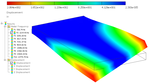
Creating a modal analysis provides the means to calculate the natural frequencies of vibration for the number of frequencies specified. It includes frequencies that correspond to rigid body movements. In an unconstrained simulation, for example, the first six modes occur at 0Hz corresponding to the six rigid body movements. Design constraints can be geometry based or a frequency.
You can animate the deformed shape to show the modal shape associated with a particular frequency. The contours represent relative displacement of the part as it vibrates. Mode shape images are helpful in understanding how a part or an assembly vibrates, but do not represent actual displacements. To find all the mode shapes below a given frequency, be sure to determine the next two or three mode shapes.
The Compute Preloaded Modes option runs a structural static simulation first and determines the stresses, and then computes the modes, given the prestressed condition. Without the option selected, the program ignores any structural loads defined for the frequency simulation.
After a simulation is run, the graphics region updates to display the results for the analysis type in the form of a volume plot (default display). The various results types populate the Results browser folder. To see the variety of results you can view, expand the Results folder.
| Simulation Type | Result displayed |
| Static Analysis | Displays the Von Mises Stress plot |
| Modal Analysis | Displays the first frequency mode. |
To view a different result, right-click the browser node corresponding to the results you want to see and click Activate, or, double-click the result browser node. The graphics region updates to display the selected results type.
There are several display options available for interpreting the simulation results.
The graphics region displays a volume plot and a color bar displays the range of the variable showing in the graphics region. Color order is as follows, from high values to low values: red, orange, yellow, green, cyan, and blue.

Parametric Study Configurations
For Parametric Studies, you can move sliders in the Parametric Table to display the different configurations. If the configuration was not generated, the message “Not Available” displays in the graphics region. You can right click the parameter row and select Generate Single Configuration, or run the simulation to solve the configuration.
Smooth Plot
Smooth shading is the default plot presentation for all result types, whether Static or Modal analysis simulation. Colors blend from one to the next.
Contour Plot
The contour plot presents the colors using a strict banding method. Color separation is clearly seen.
Change the shaded display:
- In the Display panel, click the Shaded Display command to display the pull down list.
- Select from Smooth Shading, Contour Shading, and No Shading. The graphics region updates.
Mesh
At any time, you can click Mesh View to overlay the mesh on the volume plot. The Mesh View command is an On/Off display toggle once the mesh has been defined.
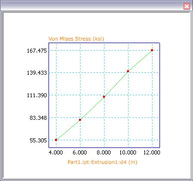
With parametric studies, you can view the results as a two-dimensional XY plot.
- In the browser, select the Results type (Von Mises Stress, Displacement, and so on) you are interested to see in a plot.
- Right-click the parameter row and click XY Plot. A window with the XY Plot is displayed over the graphics region. The window is resizable.
The following image is from the same simulation as the preceding image. However, the XY Plot is for Displacement results rather than Von Mises Stress.
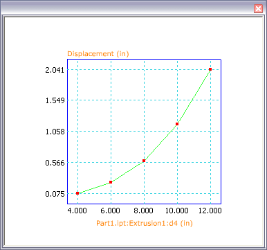
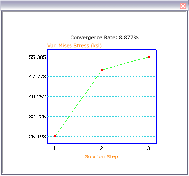
You define the convergence criteria that is used to reach a solution. You can then view the resulting convergence plot which shows the number of refinements used and the parameter values associated with each refinement.
To view an XY plot of the result convergence, you must have edited the Convergence Settings and set the Maximum Number of h Refinements to greater than zero. Right-click the Results folder node in the browser, and click Convergence Plot. The convergence criteria is set in the Convergence Settings dialog box.
- In the Prepare panel, click Convergence Settings. The dialog box displays.
- Specify the Stop Criteria percent of convergence required.
- Specify the Results type on which to converge.
- Specify any Geometric Selections
- Specify the Maximum Number of h Refinements to use.
- Specify the h Refinement Threshold.
- In the Solve panel, click Simulate. Let the simulation complete.
- In the Result panel, click Convergence Plot. The plot is displayed in a window over the graphics region.
Most often, the true geometry deformation is slight in comparison to the overall model size. In order to understand where deformation is occurring an automated exaggeration effect is provided. The Adjust Displacement Display command provides the following display options:
- Undeformed
- Actual
- Adjusted x0.5
- Adjusted x1
- Adjusted x2
- Adjusted x5
When the volume plot is displayed, select one of the display options to exaggerate the deformation.
You can animate the simulation results and retain the animation for your records by producing video output.
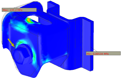
Commands for easily locating the maximum and minimum result values are located in the Display panel.
Click the Maximum Result![]() command to display an annotation at the point where this condition occurs.
command to display an annotation at the point where this condition occurs.
Click the Minimum Result![]() command to display an annotation at the point where this condition occurs.
command to display an annotation at the point where this condition occurs.
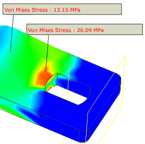
You use the Probe![]() command to identify points of interest with a label specifying the result type and value at that point. You can annotate as many points as you want. The Probe Labels
command to identify points of interest with a label specifying the result type and value at that point. You can annotate as many points as you want. The Probe Labels![]() command turns visibility on and off for those labels.
command turns visibility on and off for those labels.
The Boundary Conditions![]() command turns on and off the display of the load indicator, which points to where the load is applied.
command turns on and off the display of the load indicator, which points to where the load is applied.
To view the results for different parametric values, move the sliders on the Parametric Table. If the results of the simulations are ready for evaluation, you can display a chart for the results of each parameter or parameter change.
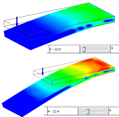
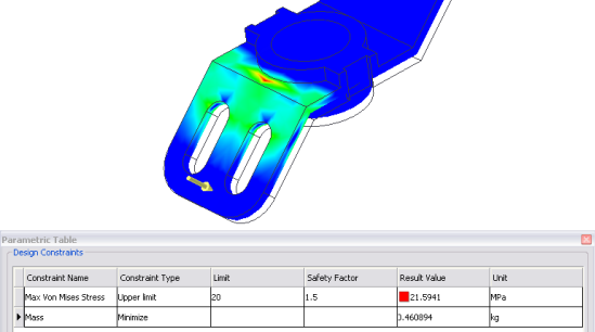
Optimize and filter results by setting limits on some constraint values and minimizing others. In the Parametric Table, Design Constraints section, set the status of a constraint to a type of limit. Specify the value and safety factor of the limit. Then change the status of another constraint to Minimize. The configuration updates and displays a result with the minimized values. If there is an existing configuration that meets all the limits, it displays. Otherwise, the result violates a constraint.
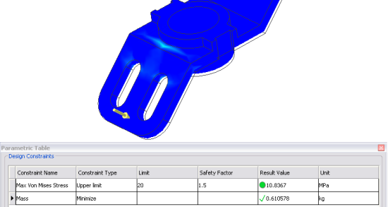
When an optimized solution displays, you can still move the sliders. The constraint values display a green check mark for the optimized constraint. For limit constraints with a safety factor, a colored shape displays to indicate if the constraint was exceeded. A green circle indicates the value lies within the acceptable range and a red square indicates the value lies outside of the acceptable range.
After running a simulation, you can see results values for given points on the model. You use the Probe command to specify the points, and the Probe Labels command to control probe label visibility.
After running a simulation, probe a point:
- On the ribbon, click


 .
. - On the model, click the point of interest. A label with a leader to the point is displayed.
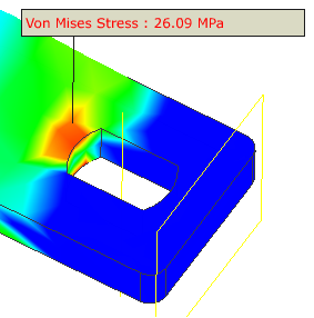
- You can probe multiple points.

- You can also manipulate labels for a clearer view of the simulation information (See Visualize Results).
Manipulate labels in the graphics window
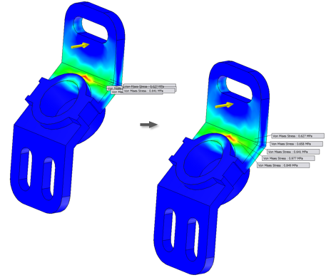
Manipulate labels in the graphics window, including labels associated with result probes, min and max values, and mesh failures, to better view and present simulation information. You can change the initial distance at which labels are placed, drag labels, and reset the position of labels.
As appropriate, you can define the initial displacement distance of the labels relative to where you click in the model:
- In the graphics window, individually- or multi-select the appropriate labels.
- Click one of the selected labels and drag to the new position.
Reset selected labels to their initial placement:
- In the graphics window, individually- or multi-select the appropriate labels.
- Right-click and select Reset Position.
To reposition all labels in the graphics window, right-click any label, and select Reset All Positions.
You can view the deformation of a part associated with a particular frequency by activating the corresponding mode plot represented by the browser node. The contours represent relative deformation of the part as it vibrates. By default, results for eight frequency modes and displacement nodes are generated.
You can animate the results and observe the displacement or stress build up over a sequence of images. The animation plays back a series of images, you determine how many, as an animation. You can record the animation.
Start an animation:
- In the Result panel, click Animate.

- In the dialog box, specify the number of Steps, analogous to images that you want to cycle through to see the displacement changes. To have a smoother or slower animation, increase the # Steps. Valid numbers range from 3 to 30 steps.
- If you do not want the original model to display in wireframe during the animation, clear the Show Original option.
- Click Record
 to create an AVI, specifying the video codec as part of that process.
 - Specify the playback Speed.
- Click Play
 to see the animation. You can pause playback.
 - Use Stop
 or click OK to end the animation playback.
When animating displacement of a parametric study, click on the slider to change the parameter value and cancel the Animate command. Change the value, and then click Animate.
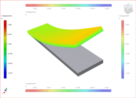
The color bar displays the range for the result being shown. The bar range is set to Automatic as the default. Inventor assigns the value range for display. The color bar is posted in the graphics region and can be relocated within the graphics region by activating the Color Bar command. Color bar display modifications are session based and do not persist between sessions.
You can modify the upper limit, lower limit, color type, and change the visibility, position, and size of the color bar.
Modify the range or position of the color bar:
- In the ribbon bar, click Color Bar
 to display the Color Bar Settings dialog box.
 - Remove the check from the Maximum and/or Minimum limit setting.
- In the Edit fields, specify a different value as the Maximum/Minimum value for the range.
- If you do not like the default position of the Color Bar, specify another position using one of the Position options.
- When finished modifying the display parameters, click OK to invoke the changes and close the dialog box.
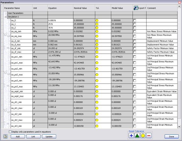
The various results from the simulation can be output as parameters in the model.
Create result parameters:
- right-click the browser Results node and click Create Result Parameters.
View results parameters:
- In the ribbon bar, click the Manage tab.
- On the Manage tab, Parameters panel, click the Parameters command. The Results Parameters are added to the list of other model parameters.
The color bar displays the range of the results being shown. The color bar is posted in the graphics region and can be relocated within the graphics region by activating the Color Bar command.
The Convergence Plot command displays the plot within a dialog box. The plot shows:
- The number of refinements required for the solution to converge, if convergence is achieved, or the number of solution steps requested for the required refinements.
- The values associated with each refinement.
The window close button in the upper right corner dismisses the dialog box.
To change the plot results criteria, right-click in any open space within the plot pane. Then, click Plot Options.
| Convergence Rate | Displays the convergence rate for the plot in the form of an XY plot. |
| Result type | Displays the selected result type. The result type is specified in the Convergence Settings dialog box. |
| Value | Displays the value range for the selected result type. |
| Solution Step | Displays the number of solution steps performed to reach the specified convergence criteria. |
Displays the Reaction Forces and Reaction Moments for the applied constraints on faces, edges, and vertices. Calculation of reaction forces includes the force acting along bounding edges and vertices. When constraints share edges or vertices, the global summation of forces could appear out of balance. The reaction forces and moments can be inconsistent if the applied constraint shares a surface, edge, or vertex with another constraint.
Access: | Simulation browser |
Reaction forces, for the Fixed, Pin, and Frictionless constraints, are displayed based on the selected constraint.
Reaction forces do not display values unless a simulation has been run. If the constraint is suppressed, the command is not enabled.
Reaction Forces are included, by default, in generated reports. You have the option to exclude this information from the report.
| Reaction Force | ||
| Total | Displays the total reaction force. | |
| X | Displays the X component reaction force. | |
| Y | Displays the Y component reaction force | |
| Z | Displays the Z component reaction force | |
| Reaction Moment | ||
| Total | Displays the total magnitude of the reaction moment about the constraint centroid | |
| X | Displays the value of the reaction moment component about the x-axis of the constraint centroid. | |
| Y | Displays the value of the reaction moment component about the y-axis of the constraint centroid. | |
| Z | Displays the value of the reaction moment component about the z-axis of the constraint centroid. | |
Especially useful for Parametric studies, Same Scale is Off by default.
When the command is on and you slide the parameter control, you see the results update immediately using a uniform scale. The color bar is scaled according to the largest and smallest values within the parameter result sets.
The other occasion where this command is useful is when you are viewing simulation results and hide component bodies. The scale remains the same and does not adjust to reflect the exclusion of the component from the view.
Animates the selected simulation results. Increase the number of steps in the playback or recording for smoother transitions between images.
Displays the simulation results for a specific point on the model.
- On the Result panel, click Probe.
- Select a point on the model.
The results for the point display in a label floating over the model with a leader to the selected point.
- You can select multiple points. Each point has a leader and label.
- Access the context menu commands to modify the label or labels in one of the following ways (See also Visualize Results):
Context menu commands
| Edit Position | Displays the Probe Coordinates dialog box. You can edit the probe position in 3D space using the X, Y, and Z coordinate values. |
| Probe Labels | By default Probe labels display when a probe is created. Click this command to toggle visibility of all probe labels. |
| Delete Probe | Deletes the selected probe. |
| Delete All Probes | Deletes all probes in the simulation. |
| Reset Position | Resets position of the selected probe. |
| Reset All Positions | Resets position of all probes in the simulation. |
You can probe multiple points of a model. For each point probed, a leader and label are displayed.
On the Display panel, click Probe Labels. The command is on by default, and is a visibility toggle. All probe points you have specified display their associated leader and label when the command is engaged. All are hidden when you disengage the command.
Output parameters of the simulation results are created on demand. The parameters are added to the model parameters and are accessed from the model parameter command. The output parameters are grouped in a folder bearing the simulation name.
Access: | Right-click the Results browser node and select Create Result Parameters. |
Use the model parameter command to access the output parameters, as you would model and user-defined parameters.
View the results parameters:
- In the ribbon bar, click the Manage tab.
- On the Manage tab, in the Parameters panel, click the Parameters command.
Displays the contents of the simulation run.
Access: | Right-click the Results browser node and select Simulation log. |